5. Thoughts on finance ¶

Here theoretical notes on finance are placed. This is the theoretical base for the development of the finance package.

Contents

Thoughts on finance

5.1. On Time, Value and dateflows ¶

Abstract:

This a presentation of basic concepts underlying financial risk. It is mainly about the concepts of time, daycount method and value. The concepts are implemented as python code.

5.1.1. Observations and Basic Concepts ¶

5.1.1.1. Observations ¶

First we have a basic observation. It is possible to go into a bank and set up a simple loan or deposit.

A simple loan or deposit is getting or placing an amount now and then at some future time repay or receive the same amount plus accumulated interest. Either way a present value is set equal to a future payment. So we have our first basic but very important modelling concept: The present value of a future cash flow.

This concept actually implies 2 new concepts: Time and value.

5.1.1.2. Time ¶

In finance the basic time measure is days or dates. On a specific date one part delivers something to the other part. This date can be specified in 2 ways:

As a specific date

As a period from a starting point, typically today

In the Python package finance there is an implementation of both banking day calculations and period calculations.

This module contains a subclass bankdate implementing the typical banking day type calculations, i.e.

adding a number (integer) of years, month or days to a bankdate

finding the difference in years, month or days for 2 bankdates

comparing 2 bankdates

finding the previous or next valid bankdate taking into account weekends and holidays

5.1.1.3. Value ¶

Wikipedia on Value: ...value is how much a desired object or condition is worth relative to other objects or conditions

Wikipedia on Money: Money is anything that is generally accepted as payment for goods and services and repayment of debts. The main functions of money are distinguished as:

A medium of exchange
A unit of account
A store of value
And occasionally, a standard of deferred payment.

So in this context anything with value is defined as money.

5.1.1.4. The drivers for setting the value of money ¶

Wikipedia on Store of Value: Storage of value is one of several distinct functions of money. ... It is also distinct from the medium of exchange function which requires durability when used in trade and to minimize fraud opportunities. ... While these items (common alternatives for storing value, the author) may be inconvenient to trade daily or store, and may vary in value quite significantly, they rarely or never lose all value. This is the point of any store of value, to impose a natural risk management simply due to inherent stable demand for the underlying asset.

Wikipedia on Risk Management: Risk management is the identification, assessment, and prioritization of risks (defined in ISO 31000 as the effect of uncertainty on objectives, whether positive or negative) followed by coordinated and economical application of resources to minimize, monitor, and control the probability and/or impact of unfortunate events or to maximize the realization of opportunities.

Basically there are 2 opposite needs driving the price process:

The need for concentrate liquidity ie sufficient surplus of value. Eg when buying a house, a firm e.t.c. ie for consumption. This is called borrowing.
The need for storing liquidity at future times. Ie for postponing consumption. This is called lending

In the following it assumes that 1 sort of money (A currency like EUR, a stock like IBM, commodities like wheat etc) is selected.

5.1.2. The law of one price and dateflows ¶

If 2 similar loan offers are presented from 2 different banks it would be expected that the present value for the 2 offers to be allmost similar as well. Otherwise the cheapest would be chosen. This is a consequence of the informed market. Hence the law of one price.

Even better, if it is possible to borrow to the cheap rate and invest to the expensive rate. That way an arbitrage is made. In theory an arbitrage is often assumed not to exist.

Definition, dateflow:

A dateflow is a set of future T ordered (after time) payments $\left(c_{t_{i}}\right)_{i=1}^{T}$ at times $\left(t_{i}\right)_{i=1}^{T}$ expressed as dates. These payments can be considered vectors. Ie. dateflows that be added and multiplied like normal vectors after filling with zeroes at missing times so that the 2 vectors have the same set of times. So in the following there will be no difference between vectors with ordered keys and dateflows.

The maturity of a dateflow is the biggest time with a non-zero payment.

The concept of dateflows are implemented in the Python module dateflow. The times in the dateflow are based of concept banking day described above.

The class dateflow is a set of 1 or more pairs of a bankdate and and a (float) value. The operations are

adding 2 dateflows
multiplying a dateflow with a number
removing excessive pairs (identified by a list bankdate of bankdates)

Example:

Consider a time vector $\overrightarrow{a}=\left(\begin{array}{ccc}1, & 2, & 3\end{array}\right)$ at times $\left(\begin{array}{ccc} 2, & 3, & 4\end{array}\right)$ and a time vector $\overrightarrow{b}=\left(\begin{array}{ccc}4, & 5, & 6\end{array}\right)$ at times $\left(\begin{array}{ccc}1, & 3, & 5\end{array}\right)$ .

In order to add, subtract or multiply $\overrightarrow{a}$ and $\overrightarrow{b}$ they must first have the same set of times, ie. $\left(\begin{array}{ccccc}1, & 2, & 3, & 4, & 5\end{array}\right)$ . Then eg.

$\begin{eqnarray*} \overrightarrow{a}+\overrightarrow{b} & = & \left(\begin{array}{ccccc}0, & 1, & 2, & 3, & 0\end{array}\right)+ \left(\begin{array}{ccccc}4, & 0, & 5, & 0, & 6\end{array}\right)\\ & = & \left(\begin{array}{ccccc}4, & 1+0, & 2+5, & 3+0, & 6\end{array}\right)\\ & = & \left(\begin{array}{ccccc}4, & 1, & 7, & 3, & 6\end{array}\right) \end{eqnarray*}$

Definition, positive vector:

A vector $\vec{v}=\left(v_{i}\right)_{i=1}^{n}\in\mathbb{R}^{n}$ is a row vector and $\vec{v}\geq0\Leftrightarrow v_{i}\geq0\:\forall i\in\left\{ 1,\ldots,n\right\}$ ie all vector values are nonnegative $\vec{v}>0\Leftrightarrow v_{i}\geq0\:\forall i\in\left\{ 1,\ldots,n\right\}\wedge\exists i:v_{i}>0$ ie all vector values are nonzero and at least one vector value is positive $\vec{v}\gg0\Leftrightarrow v_{i}>0\:\forall i\in\left\{ 1,\ldots,n\right\}$ ie all vector values are positive

Off course the definition for negative values is similar, ie:

$\vec{v}\leq0\Leftrightarrow-\vec{v}\geq0, \vec{v}<0\Leftrightarrow-\vec{v}>0$ and $\vec{v}\ll0\Leftrightarrow-\vec{v}\gg0$

It is possible to sell dateflows in order to recieve a (positive) price now and vice versa.

Definition, financial market:

Consider a selection of N dateflows (dateflow). Every dateflow can be traded at a price $\pi$ .

A financial market is the set of $\left(\vec{\pi}^{\intercal},\bar{C}\right)$ where $\vec{\pi}^{\intercal}\in\mathbb{R}^{N}$ is a columnvector of nonzero prices.

And $\bar{C}$ is a $N \times T$ matrix where each row is a dateflow and all dateflows has been filled with the necessary zeroes so that all dateflows has a value for all dateflow times.

A financial market can be considered as a set of related dateflow instruments, eg in the same currency and/or in a specified timespan.

Definition, portfolio:

A portfolio is a set of amounts of dateflows from a financial market. A portfolio $\vec{\theta}, \vec{\theta}\in\mathbb{R}^{N}$ , has dateflow $\vec{\theta}\cdot\bar{C}$ and price $\vec{\pi}\cdot\vec{\theta}^{\intercal}$ or $\vec{\theta}\cdot\vec{\pi}^{\intercal}$ .

Lemma (Stiemke’s Lemma):

Let $\bar{A}$ be a $n \times m$ matrix. Then exactly one of the following statements are true:

$\begin{eqnarray} \quad\exists\vec{x}\in\mathbb{R}^{m}, \vec{x}\gg0 : \bar{A}\cdot\vec{x}^{\intercal}=0 \\ \quad\exists\vec{y}\in\mathbb{R}^{n} : \vec{y}\cdot\bar{A}>0 \end{eqnarray}$

Proof:

Assume they both are true. Then $\exists\vec{y}\in\mathbb{R}^{n},\exists\vec{x}\in\mathbb{R}^{m},\vec{x}\gg0 : \vec{y}\cdot\left(\bar{A}\cdot\vec{x}^{\intercal}\right)=0$

and

$\vec{y}\cdot\bar{A}>0$

This can’t be true because $\vec{x}\gg0$ and $\vec{y}\cdot\bar{A}>0$

means that $\vec{y}\cdot\left(\bar{A}\cdot\vec{x}^{\intercal}\right)>0$ .

Hence the two statements can’t be true at the same time.

Now assume that they are both false, ie

$\forall\vec{y}\in\mathbb{R}^{n},\forall\vec{x}\in\mathbb{R}^{m},\vec{x}\gg0 : \bar{A}\cdot\vec{x}^{\intercal}\neq0$ and $-\vec{y}\cdot\bar{A}>0$

And again since $\vec{x}\gg0$ and $-\vec{y}\cdot\bar{A}>0$ means that $\left(-\vec{y}\cdot\bar{A}\right)\cdot\vec{x}^{\intercal}>0\forall\vec{y}$ .

But every vector $\vec{z}\in\mathbb{R}^{n}$ in the orthogonal subspace of $\bar{A}\cdot\vec{x}^{\intercal}$ will give $\left(-\vec{y}\cdot\bar{A}\right)\cdot\vec{x}^{\intercal}=0$ .

Contradiction again, meaning that at precisely one of the statements must be true.

Q.E.D.

Definition, arbitrage:

An portfolio $\vec{\theta}$ is an arbitrage if either the price of the portfolio is zero, ie $\vec{\theta}\cdot\vec{\pi}^{\intercal}=0$ and the dateflow is positive at at least one future point, ie $\vec{\theta}\cdot\bar{C}>0$ or if the price is negative (giving money to the owner right away) ie. $\vec{\theta}\cdot\vec{\pi}^{\intercal}<0$ and maybe also gives the owner a future dateflow, ie. $\vec{\theta}\cdot\bar{C}\geq0$ .

In short a portfolio is an arbitrage iff $\left(-\vec{\theta}\cdot\vec{\pi}^{\intercal},\vec{\theta}\cdot\bar{C}\right)=\vec{\theta}\cdot\left(-\vec{\pi}^{\intercal},\bar{C}\right)>0$ .

A financial market $\left(\vec{\pi}^{\intercal},\bar{C}\right)$ is arbitragefree iff there is no arbitrage portfolio in the market.

Theorem, arbitragefree financial market:

A financial market $\left(\vec{\pi}^{\intercal},\bar{C}\right)$ is arbitragefree iff there exists a strict positive price vector $\vec{d}\in\mathbb{R}_{+}^{T}$ such that $\vec{\pi}^{\intercal}=\bar{C}\cdot\vec{d^{\intercal}}$ . Here $\vec{d}$ is refered to as the discount vector.

Proof:

From definition of an arbitrage we have:

A financial market $\left(\vec{\pi}^{\intercal},\bar{C}\right)$ is arbitragefree iff there is no arbitrage portfolio in the market.

A portfolio is an arbitrage iff $\left(-\vec{\theta}\cdot\vec{\pi}^{\intercal},\vec{\theta}\cdot\bar{C}\right)=\vec{\theta}\cdot\left(-\vec{\pi}^{\intercal},\bar{C}\right)>0$ .

So there can be no portfolio such that $\vec{\theta}\cdot\left(-\vec{\pi}^{\intercal},\bar{C}\right)>0$ . According to Stiemke’s lemma $\exists\vec{x}\in\mathbb{R}^{T},\, x_{0}\in\mathbb{R}, \vec{x}\gg0 :\left(-\vec{\pi}^{\intercal},\bar{C}\right)\cdot\left(x_{0},\vec{x}\right)^{\intercal}=0\Leftrightarrow\bar{C}\cdot\vec{x}^{\intercal}=\vec{\pi}^{\intercal}\cdot x_{0}$ .

Hence $\vec{d}=\frac{1}{x_{0}}\cdot\vec{x}$

Q.E.D.

Definition, complete financial market

A financial market $\left(\vec{\pi}^{\intercal},\bar{C}\right)$ is complete iff for all discount vectors $\vec{y}\in\mathbb{R}^{T}$ there exists a vector $\vec{x}\in\mathbb{R}^{N}$ such that $\vec{x}\cdot\bar{C}=\vec{y}\Leftrightarrow\bar{C}^{\intercal}\cdot\vec{x}^{\intercal}=\vec{y}^{\intercal}$ .

From linear algebra it is known that a necessary condition for a market market to be complete is that $N \geq T$ , ie the number of dateflow in the financial market must exceed the number of time points to discount.

A mathematical definition a financial market being complete is that the function $f\left(\vec{x}\right)=\bar{C}^{\intercal}\cdot\vec{x}^{\intercal}$ is surjective.

In words completeness happens when there are more instruments than prices.

Theorem, existence of discount factors

Let a financial market $\left(\vec{\pi}^{\intercal},\bar{C}\right)$ be arbitrage free. Then it is complete iff there exists a unique vector of discount factors.

Proof:

Assume first completeness.

First find the vectors $\vec{z_{t}}\in\mathbb{R}^{N}$ that has the unity vector $\vec{e_{t}}$ , ie $\vec{z_{t}}\cdot\bar{C}=\vec{e_{t}}$ . They exist due to completeness.

$\bar{Z}$ is a $T \times N$ matrix having $\vec{z_{t}}$ as row vectors and rank T, $T \leq N$ .

Then we have $\bar{Z}\cdot\bar{C}=\bar{I}$ and $\vec{\pi}^{\intercal}=\bar{C}\cdot\vec{d^{\intercal}}\Leftrightarrow\bar{Z}\cdot\vec{\pi}^{\intercal}=\vec{d^{\intercal}}$ and hence that there can be only 1 vector of discount factors.

Now assume the uniqueness of the vector of discount factors.

Further assume that the market is not complete. Then there exists a nonzero vector $\vec{z}\in\mathbb{R}^{T}$ such that $\bar{C}\cdot\vec{z}^{\intercal}=\vec{0}$ . Choose a number a such $\vec{d^{\intercal}}-a\cdot\vec{z^{\intercal}}\gg0$ . This is a second vector of discount factors which is a contradiction.

Q.E.D.

Definition, zero bonds:

The dateflow of a zero bond at time t has value 1 at time t. Hence in a financial market the dateflow of a zero bond is a unit vector $\vec{e_{t}}\in\mathbb{R}^{T}$ where the only nonzero value, 1, is at the place reserved for time t.

Theorem, discount factor base for a financial market

Assume an arbitrage free and complete financial market. Let $\vec{d}$ be the unique discount vector. Then the price of a zero bond at time t is $d_{t}$ , the discount factor reserved for time t.

Proof:

First find the portfolio $\vec{\theta_{t}}$ that has the dateflow $\vec{e_{t}}$ , ie $\vec{\theta_{t}}\cdot\bar{C}=\vec{e_{t}}$ . It exist due to completeness.

The price for the dateflow is:

$\vec{\theta}_{t}\cdot\vec{\pi}^{\intercal}=\vec{\theta}_{t}\cdot \bar{C}\cdot\vec{d^{\intercal}}=\vec{e_{t}}\cdot\vec{d^{\intercal}}=d_{t}$

Q.E.D.

A consquence of the theorem is that every instrument is to be considered as a portfolio of zero bonds thus making a financial market and portfolios herein to portfolios of zero bonds.

It is possible theoretically to carry on with the concept of a financial market $\left(\vec{\pi}^{\intercal},\bar{C}\right)$ . The problem is that $\bar{C}$ soon becomes very big. But ussually the market is not complete.

The number of columns (T) might correspond to every day in mayby 30 or 50 years and the problem is to find at least the same amount of trades in order to calculate the discount factors.

The essence of the above theorem is that there is a close connection between zero bonds and discount factors. That prices are only dependent on duration before repayment.

Therefore it would be far better to consider a function which gives a discount factor given a time t. The function would typically have a few parameters and this makes the estimation based on trades much easier.

Definition, discount (factor) function

A discount (factor) function returns the price for every future zero bonds when there is a zero bond for every future date.

5.1.3. Discount factor functions ¶

5.1.3.1. On discount factors and rates on a minimum period ¶

From the previous chapter the building stones for modeling a discount function is presented.

First the notion of a financial market, ie. the model is limited to a set of dateflows. These dateflows stems from a set of comparable trades, a notion not yet defined.

It is reasonable to assume that there are no arbitrage in a system since no one wants to give away money. This implies a strict positive price function.

Also even though the markets typically aren’t complete the zero bonds will be used as a base for developing a discount function. This function is assumed to be unique for a market.

In the model above it is assumed that there is a zero bond for each minimum period in the future. This means that the market is complete, so this assumption needs to be relaxed at some point.

As a strange thing the modelling of the discount function is based on the rate concept, ie the loss in value for a future payment quoted in relation to now. In every other financial quotes one quotes the value of one thing in relation to the value of something else. Eg USD is qouted in relation EUR or vice versa, and the IBM stock is quoted in USD etc. In the end whats matters is what value a future payment has, ie the discount function? And with what certainty or risk the future has?

Anyway we need to introduce the concept of rate now. Spot rate is the rate observed this very minut. Typically some compounded spot rate or a compounded forward rate. Later we will go further in the definitions of rate.

It is only because prices for future payments are quoted based on rates that we choose to work with rates and not discount values alone.

Definition, scalable discount function:

A discount function is scalable if $d_t = d(t)=\prod_{i=0}^{t}df_{i}$ where $df_{i}$ is the future discount factor for the minimum period number i. When observed in the market $d(t)$ is the discrete time compounded spot price for a zero bond.

A consequence is that the future discount factor for a period from time $t_{1}$ to time $t_{2}, t_{1} < t_{2}$ can be expressed as $d(t_{1},t_{2})=\prod_{i=t_{1}}^{t_{2}}df_{i}$ . Note that $d(t)=d(0,t)$ . When observed in the market $d(t_{1},t_{2})$ is the discrete time compounded forward price for a zero bond.

The minimum period might be a day. Sometimes it make more sense to use minimum periods like a month, a quarter or a year.

In the special case where all the $df_{i}$ ‘s are equal the discrete time compounded forward price for a zero bond is

$d(t_{1},t_{2}) &= \prod_{i=t_{1}}^{t_{2}}df\\ &= df^{(t_{2} - t_{1})}$

When borrowing or lending it is expected at least to repay the amount borrowed or lended. Futher it is expected that there is an earning and/or a cost coverage for having excessive liquidity now. This earning is called the rate and is the price for borrowing.

It is quite easy to see that

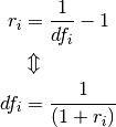
$r_{i} &= \frac{1}{df_{i}} - 1 \\ & \Updownarrow \\ df_{i} &= \frac{1}{\left(1+r_{i}\right)}$

where $r_{i}$ is the price for borrowing one day at day i from now. Since prices usually are positive, it means that usually $0<df_{i}\leq1$ .

In the special case of constant rate discrete time compounded forward price for a zero bond is

$d(t_{1},t_{2}) = (1 + r)^{-(t_{2} - t_{1})}`$

which the standard textbook formula for discounting using the Bond rate convention.

The rate can be formulated in different ways:

discrete time versus continuous time

Continuously compounded discrete rate

Forward rate

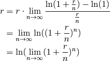
Instantaneous rate occurs when the minimum period converges to zero for the bond rate ie: $e^r = \lim_{n \rightarrow \infty}(1+\frac{r}{n})^n$

which can be seen from

$r & = r\cdot\lim_{n \rightarrow \infty}\frac{\ln(1+\frac{r}{n}) - \ln(1)}{\frac{r}{n}} \\ & = \lim_{n \rightarrow \infty}\ln((1+\frac{r}{n})^n) \\ & = \ln(\lim_{n \rightarrow \infty}(1+\frac{r}{n})^n)$

So one way to combine discount factors and rates are though the exponential function and instantaneous rates.

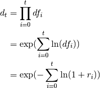
Further scalability implies that

$d_{t} & = \prod_{i=0}^{t}df_{i} \\ & = \exp(\sum_{i=0}^{t}\ln(df_{i})) \\ & = \exp(-\sum_{i=0}^{t}\ln(1+r_{i}))$

which means that a discount factor can be described though the summation or integration of the instantaneous rate.

In the special case where the instantaneous rate, ir, is constant, ie $ir = -\ln(df_i) = \ln(1 + r_i) \forall i$ then

$d_{t} & = df^{t} \\ & = \exp(-ir \cdot t)$

which is used for modelling in many finance textbooks.

Instantaneous rates are easy to manipulate when compounding so that is why they are used. However rates are usually not quoted as instantaneous rates but rather as eg bond or swap rates.

In the end it doesn’t matter what discounting and daycount (see below) which is used. In all cases it will be calibrated to marginally different parameters leading to the same set of prices.

Note

The choice here is to use instantaneous rates and continuous discounting since this is the base for most theoretical work.

5.2. Day count conventions ¶

Abstract:

Here is a very short presentation of the problem of using different time at at the same time in finance. More information on this subject will be added in time.

The problem with daily rates is that they are close to zero and especially in the old days it meant problems with rounding errors.

Further if someone is lending or borrowing over a longer periods they would prefer quotes on years, quarters or months etc.

To be able to compare rates they are typically quoted per year. To get the rate per quarter is a matter of dividing the rate quote per year with 4, the monthly rate by dividing by 12 etc.

Since days, months and year aren’t fully comparable it leads to the notion of day count conventions.

In order to do calculations it is necessary to look at time differences and the differences has to be a number. That would not cause any troubles if it weren’t for the fact that price quotes for borrowing are specified pr year, pr half a year, pr quarter of a year or pr month etc.

Days, months and years are measures of time differences of incompatible definitions, i.e. a month is the time elapsing between successive new moons (about 29.53 average days) and a year is the time required for the Earth to travel once around the Sun (about 365 1/4 average days).

Therefore it is not possible to move from one time differences measure to another, and hence the need for Day Count Conventions, see eg

QUOTES PER YEAR implies timeconversion to year fractions in order to do calculations

A class DateToTime is introduced to implement the most important day count conventions and date rolling. Also a valuationday that is chosen.

What it does is given a calculation date and the name of a day count convention it returns the time in years and fractions of years

5.3. On Yieldcurves ¶

Abstract:

In the presentation on Time and value the key subject was unique price function. Instead of talking of prices of the cashflows it is customary to talk of the price of lending, i.e. the rate or yield. Here we will look into several different types of yield curve definitions. These yield curves will be implemented in the finance package.

5.3.1. Basic concepts ¶

Note

There no implementation of calibration at this point.

Since most yieldcurve models are specified as a sum of one or more simple yield curve functions.

A yieldcurve function must be a callable class. Also a string representation must be defined showing name and used parameters.

5.3.2. The basic design for yieldcurves ¶

Here is the design and the definitions of the functionality of yieldcurve base class in the finance package.

First of all there are some generel functionality:

add_function It should be possible dynamically to add more yield curve functions to a yield curve
yieldcurve_functions Return the list of used functions
Print a yieldcurve When printed a yield curve shows the string representation for all yield curve functions

And then there are the pure calculation functionality which are defined in the subsections below.

5.3.2.1. continous_forward_rate ¶

This is the base function from which everything else is derived. At time t it is the average rate from now till then.

Warning

Since this is the base a future estimation/calibration procedure must also be based on continous_forward_rate. I.e. this is the function that needs to be optimized.

5.3.2.2. continous_rate_timeslope ¶

The continous_rate_timeslope is the first order derivative with regard to time. It is used in others calculations. The formula is:

$continous\_rate\_timeslope(t) = \frac{\partial continous\_forward\_rate(t)}{\partial t}$

5.3.2.3. instantanious_forward_rate ¶

Actually in all textbooks and articles the continous_forward_rate is defined by as the average over time of the instantanious_forward_rate.

But for computational purposes it is better to reverse it. So by definition:

$continous\_forward\_rate(t) = \frac{1}{t}\int_{0}^{t}instantanious\_forward\_rate(x)\partial x$

And then it follows:

$instantanious\_forward\_rate(t) &= \frac{\partial \left(t \cdot continous\_forward\_rate(t)\right)}{\partial t} \\ &= continous\_forward\_rate(t) \\ & \quad + t \cdot \frac{\partial continous\_forward\_rate(t)}{\partial t} \\ &= continous\_forward\_rate(t) \\ & \quad + t \cdot continous\_forward\_timeslope(t)$

5.3.2.4. discount_factor ¶

The discount_factor is giving the present value of the amount of 1 unit at a future time t, P(t). And the formula is:

$P(t) &= \exp\left(-\int_{0}^{t}instantanious\_forward\_rate(x)\partial x\right) \\ &= \exp\left(-continous\_forward\_rate(t) \cdot t\right)$

When a yieldcurve is called as a python function the yieldcurve will return the discount_factor.

5.3.2.5. zero_coupon_rate ¶

The definition of zero_coupon_rate comes from the bond and deposit market. It is a bit like the continous_forward_rate except for how the discounting is done. Here the discount_factor is:

$P(t) = \left(1 + zero\_coupon\_rate\right)^{-t}$

Combining the definition of the discount_factor and the zero_coupon_rate one gets:

$\exp\left(-continous\_forward\_rate(t) \cdot t\right) = \left(1 + zero\_coupon\_rate\right)^{-t}$

or:

$continous\_forward\_rate(t) = \ln\left(1 + zero\_coupon\_rate\right)$

So there is a simple relation between the continous_forward_rate and the zero_coupon_rate. The reverse formula is:

$zero\_coupon\_rate = \exp (continous\_forward\_rate(t)) - 1$

5.3.2.6. discrete_forward_rate ¶

The discrete_forward_rate is the average rate between 2 future times $t_1$ and $t_2$ . The forward rate is defined as (using no arbitrage):

$(1 + zero\_coupon\_rate(t_2))^{t_2} &= (1 + zero\_coupon\_rate(t_1))^{t_1} \\ & \quad \cdot (1 + discrete\_forward\_rate(t_1, t_2))^{t_2 - t_1}$

Taking the log gives:

$& continous\_forward\_rate(t_2) \cdot t_2 = \\ & \quad continous\_forward\_rate(t_1) \cdot t_1 \\ & \quad + \ln (1 + discrete\_forward\_rate(t_1, t_2)) \cdot (t_2 - t_1)$

or

$& discrete\_forward\_rate(t_1, t_2) = \\ & \quad \exp \left(\frac{continous\_forward\_rate(t_2) \cdot t_2 - continous\_forward\_rate(t_1) \cdot t_1}{t_2 - t_1}\right) - 1$

This way the discrete_forward_rate is the descretized time weighted average of the continous_forward_rate.

Note

If one of the times are zero then formula reduces to the formula for the zero_coupon_rate

5.3.3. Addding a Parallel Shift or a spread ¶

Since quotes typically are for the zero_coupon_rate then it makes most sence to define a parallel shift, additive_shift to the zero_coupon_rate giving:

$continous\_forward\_rate(t, additive\_shift) = \ln\left(1 + zero\_coupon\_rate + additive\_shift\right)$

On the other the uses of shift often requires one to find the shift that gives a cashflow a certain target value. In that case it is more feasable to add a shift to the continous_forward_rate. This type will be called a multiplicative shift. It is worth noting that in many textbooks and articles where the authors uses a continous compounding then a shift will be multiplicative.

The reason for the name multiplicative_shift is:

$P(t, multiplicative\_shift) &= \exp\left(-(continous\_forward\_rate(t) + multiplicative\_shift) \cdot t\right) \\ &= \exp\left(-continous\_forward\_rate(t) \cdot t\right) \cdot \exp\left(-multiplicative\_shift \cdot t\right) \\ &= \left(1 + zero\_coupon\_rate\right)^{-t} \cdot \left(1 + \left(\exp(multiplicative\_shift) - 1)\right)\right)^{-t} \\ &= \left(1 + zero\_coupon\_rate\right)^{-t} \cdot \left(1 + multiplicative\_shift\_rate\right)^{-t} \\ &= P(t) \cdot \left(1 + multiplicative\_shift\_rate\right)^{-t}$

Here $multiplicative\_shift\_rate = \exp(multiplicative\_shift) - 1$ .

Note

So now it becomes obvious why the multiplicative shift is mathematically more feasable than the additive. This is because the multiplicative_shift_rate is independent of the original yieldcurve when discounting or compounding.

In other words the discounting can be done in 2 steps, first discount the cashflows with regard to yieldcurve and discount the discount the discounted cashflows with regard to a simple yieldcurve with a constant rate (the multiplicative_shift_rate).

Anyway the additive_shift cannot be ignored since there are quotes related to it.

The relationship between the additive_shift and the multiplicative_shift_rate can be seen from looking at the discount factors for a specific future time t expressed though the zero_coupon_rate:

$\left(1 + zero\_coupon\_rate + additive\_shift\right)^{-t} &= \left(1 + zero\_coupon\_rate\right)^{-t} \cdot \left(1 + multiplicative\_shift\_rate\right)^{-t} \\ & \Updownarrow \\ additive\_shift &= multiplicative\_shift\_rate \cdot (1 + zero\_coupon\_rate)$

Note however that when additive_shift and multiplicative_shift_rate are calculated for more complex cashflows (ie more than 1 payment) then the relation isn’t that simple.

5.3.4. On the Nelson Siegel yieldcurve ¶

5.3.4.1. Derivation of the Nelson Siegel ¶

Nelson and Siegel says that the Expectation theory of the term structure of interest rates leads to an heuristic motivation of their yieldcurve model. This is because if the spot rates are given by a differential equation then the forward rates would be generated by the solution to this differential equation. The next thing is to identify a proper differential equation. And the choice ends at a linear second order differential equation with 2 real and unequal roots.

So the instantanious forward rate r(t) would be:

$r(t) = \beta_0 + \beta_1 \cdot \exp(-\frac{t}{\tau_1}) + \beta_2 \cdot \exp(-\frac{t}{\tau_2})$

leading to 5 parameters to be estimated. Nelson and Siegel carry on with experimenting and they find that this model was overparameterized. This might not come as a surprise since the solution is build on the sum of 2 versions of the very same function. The parameter estimates might become highly correlated.

The authors then turn to the case with 1 real root and the instantanious forward rate becomes:

$r(t) = \beta_0 + \beta_1 \cdot \exp(-\frac{t}{\tau}) + \beta_2 \cdot \frac{t}{\tau} \cdot \exp(-\frac{t}{\tau})$

Then the continous forward rate R(t) (using the original notation) becomes:

(1) $R(t) & = \frac{1}{t}\int_{0}^{t}r(x)\partial x \\ & = \frac{1}{t}\int_{0}^{t}\beta_{0} + \beta_{1} \cdot \exp(-\frac{x}{\tau}) + \beta_{2} \cdot \frac{x}{\tau} \cdot \exp(-\frac{x}{\tau}) \partial x \\ & = \frac{1}{t} \cdot \left(\beta_{0} \cdot t - \beta_{1} \cdot \tau \cdot \left(\exp(-\frac{t}{\tau}) - 1\right) + \beta_{2} \cdot \left( -t \cdot \exp(-\frac{t}{\tau}) - \tau \cdot \left(\exp(-\frac{t}{\tau}) - 1\right)\right)\right) \\ & = \beta_{0} + \beta_{1} \cdot \frac{1 - \exp(-\frac{t}{\tau})}{\frac{t}{\tau}} + \beta_{2} \cdot \left( \frac{1 - \exp(-\frac{t}{\tau})}{\frac{t}{\tau}} - \exp(-\frac{t}{\tau})\right)$

Note

The derivation of the formula (1) above is based on a continous forward rate setup otherwise you couldn’t talk about instantanious forward rate

Note

Some authors chooses this representation for the Nelson Siegel yieldcurve. This way $\beta_0$ is interpreted as the level of the curve, the magnitude of the slope is $\beta_1$ and finally $\beta_2$ is the magnitude of the curvature. $\tau$ is representing a time rescale.

By looking at the parts of the instantanious forward rate Nelson and Siegel interpretes $\beta_0$ as the long term rate $\beta_1$ is the short term rate contribution while $\beta_2$ as the medium term rate.

Other authors including Nelson and Siegel chooses to simplify the Nelson Siegel formula by a reparametrisation:

$R(t) = \beta_{0} + \left(\beta_{1} + \beta_{2}\right) \cdot \frac{1 - \exp(-\frac{t}{\tau})}{\frac{t}{\tau}} + \beta_{2} \cdot \left(-\exp(-\frac{t}{\tau})\right)$

It is mathematically simpler. But then there is no financial interpretation of the parameters.

Due to the financial interpretation of the $\beta$ ‘s the code in the package finance and the rest of this text is based on on the first formula (1).

It is fairly easy to see:

$\lim_{t \rightarrow \infty} R(t) = \beta_0$ so $\beta_0$ is the long term rate
$\lim_{t \rightarrow 0} R(t) = \beta_0 + \beta_1$ so $\beta_0 + \beta_1$ is the rate at time 0. Hence $\beta_1$ represents the pure short rate contribution. And hence is the $\beta_2$ the medium time range rate contribution
Also the factors of both $\beta_1$ and $\beta_2$ converges to 0 and each others as time becomes large
When $\tau$ is large the time axis is stretched and so is the difference between the factors of $\beta_1$ and $\beta_2$

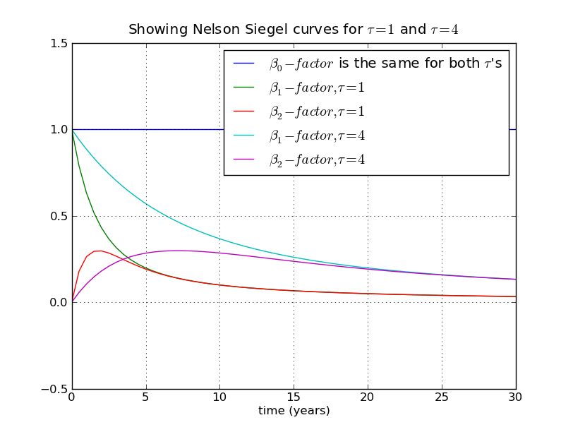
This is also shown in the graph below (where $\tau$ = 4):

The graph is made in pyplot as:

'''Code for generating a graph showing the effect of the different factors in
Nelson Siegel
'''

import matplotlib.pyplot as plt
import decimalpy as dp
import finance as fn

ns = ns = fn.yieldcurves.NelsonSiegel(1, 1, 1, 1)
tau_list = dp.Vector([1, 4])
legend_list = [r"$\beta_0-factor$ is the same for both $\tau$'s"]
xdata = dp.Vector(range(61)) * 0.5
b0_factor = dp.Vector(61, 1)

plt.plot(xdata, b0_factor)
for tau in tau_list:
    ns.scale = 1 / tau
    plt.plot(
        xdata, ns.Slope(xdata),
        xdata, ns.Curvature(xdata)
    )
    for fac in (1,2):
        legend_list.append(r'$\beta_%s-factor, \tau = %s$' % (fac, tau))

tau_in_title = ' and '.join([r'$\tau = %s$' % x for x in tau_list])
plt.title(r'Showing Nelson Siegel curves for %s' % tau_in_title)
plt.xlabel('time (years)')
plt.grid(True)
plt.ylim(-0.5,1.5)
plt.legend(legend_list)
plt.show()

download:	the code for the Nelson Siegel graph

Observation:

This graph leads to an interesting observation on $\tau$ . When $\tau = 1$ then the difference between the factors of $\beta_1$ and $\beta_2$ is relatively small when time is greater than 5. Both factors still contribute, but there are almost no difference between them.

When $\tau = 4$ the time has to be greater than 20 before the same happens.

Is it possible to estimate $\tau$ by saying that there should be no or rather a specified small difference between the factors of $\beta_1$ and $\beta_2$ when time is greater than a specified time?

5.3.4.2. Calibration ¶

It is quite simple to set up a calibration routine if a set of points (i.e. times and rates) from zero coupons is present. This is of course no little matter to get these points.

The idea is to keep $\tau$ fixed and then do a simple regression on the times put into the factor functions from the Nelson Siegel formula (1).

To find the optimal $\tau$ use a algorithm to find the minimum of eg. R² as a function of $\tau$ or to use observation above.

5.3.4.3. Conclusion ¶

There are no or very litle financial theory to back up the use of the Nelson Siegel. But it is simple and robust.

5.3.5. On Cubic and Financial Splines ¶

The derivation of both the natural and the financial cubic splines are shown at other places.

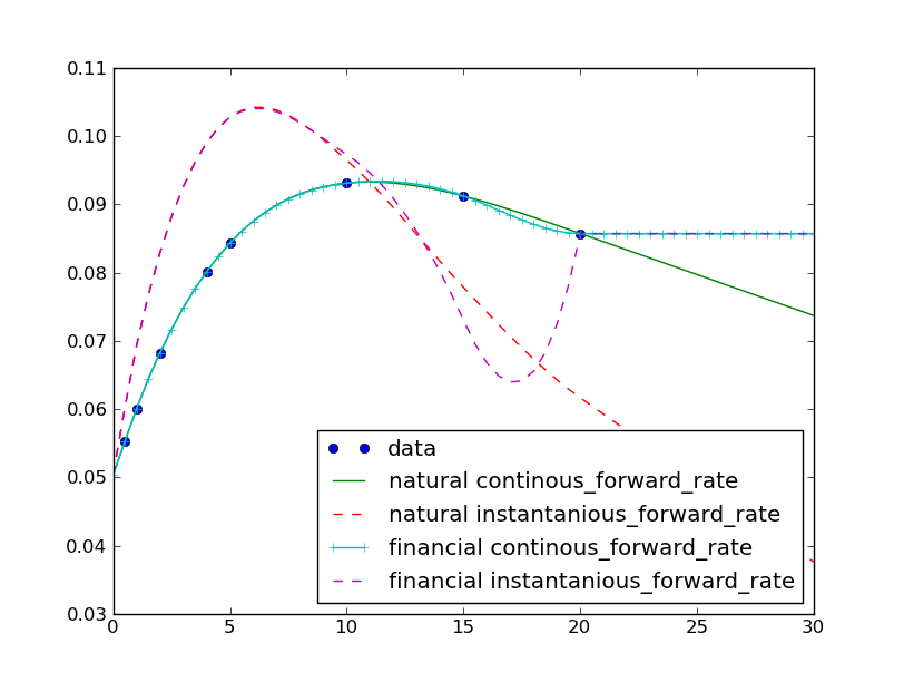
Using finance and matplotlib makes it easy to show plots on yieldcurves. The data are from [Adams]:

>>> times = [0.5, 1, 2, 4, 5, 10, 15, 20]
>>> rates = [0.0552, 0.06, 0.0682, 0.0801, 0.0843, 0.0931, 0.0912, 0.0857]

Then define the functions using finance. First the natural cubic spline:

>>> import finance
>>> f1 = finance.yieldcurves.NaturalCubicSpline(times, rates)

And then the financial cubic spline:

>>> f2 = finance.yieldcurves.FinancialCubicSpline(times, rates)

Then to do the plot below just do:

>>> import matplotlib.pyplot as plt
>>> plt.plot(times, rates, 'o',
...         times, f1.continous_forward_rate(times), '-',
...         times, f1.instantanious_forward_rate(times), '--',
...         times, f2.continous_forward_rate(times), '-+',
...         times, f2.instantanious_forward_rate(times), '--'
...         )  
>>> plt.legend(['data',
...             'natural continous_forward_rate',
...             'natural instantanious_forward_rate',
...             'financial continous_forward_rate',
...             'financial instantanious_forward_rate'
...             ], loc='best')  
>>> plt.show()

../_images/splines_zeros_and_forwards.png

In [Adams] the key point is that there are some financial inconvieniences at the extrapolations beyond the points to the right.

The natural cubic spline is extrapolated as a straight line from the end point where the line has the same slope as the curvature at the end point. In cases like the plot above this leads eventually to negative zero rates as well as forward rates.

From a financial viewpoint this not acceptable. Therefore the alternative the financial cubic splines is defined. The idea is here to secure non negative both zero and forward rates. This is done by extrapolating from the end point as a horizontal line. This way both zero and forward rates are constant from the end point. The price paid here is strange curvature as seen on the plot above. This leads to inacceptable forward prices.

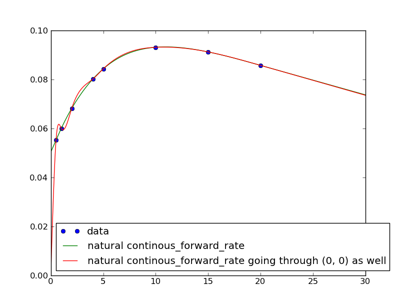
Another smothness problem arises from the points not being “placed nicely” next to each other. This can eg. be seen for the natural cubic spline by adding a (0, 0) point to (times, rates), ie:

>>> f1 = finance.yieldcurves.NaturalCubicSpline(times, rates)
>>> f2 = finance.yieldcurves.NaturalCubicSpline([0] + times, [0] + rates)
>>> plt.plot(times, rates, 'o',
...          times, f1.continous_forward_rate(times), '-',
...          times, f2.continous_forward_rate(times), '-'
...          )  
>>> plt.legend(['data',
...             'natural continous_forward_rate',
...             'natural continous_forward_rate going through (0, 0) as well'
...             ], loc='best')  
>>> plt.show()

to get the following plot:

Again here the “strange” curvature leads to inacceptable prices, eg that prices just before time 1 is higher than they are at time 1.

In order to remedy this some authors suggests a curvature penalty function when estimating. Also some suggests fewer and other time points than the ones offered by the instruments used for estimating.

This way though the splines looses their greatest advantage, ie that the splines goes through the points and near by the points.

5.3.6. Where to get Yield Curve Data ¶

To calibrate yieldcurves yield curve points are needed in the diffent currencies. Some of these data are free, eg:

U.S. Department of the Treasury

Euro area yield curve

Bank of England yield curve

It is not always easy to get data like this. For eg. commodities and equities one probably has to build yield curves eg from benchmark instruments using bootstrapping.

5.3.7. Yield Curve Derivatives ¶

This section will be elaborated later. For now it is best to study eg. Wikipedia and the references therein.

5.4. A Note on Classical Interest Rate Risk and Risk Management ¶

Abstract:

A summary of classical Interest Rate risk and risk management. It is inspired by [Bierwag], [Christensen], [delaGrandville], [Fabozzi], [FabozziKonishi] and wikipedia.

At first it is assumed that there is constant calculation rate $r_0$ for all time periods of length 1, it is a flat yield curve and the discount factors (see `Day count conventions and discount factor functions`_) are $(1+r_0)^{-t_i}$ .

Based on the definition of dateflow we now consider dateflows/cashflows as future payments $(c_i)^n_{i=1}$ at times (dates) $(t_i)^n_{i=1}$ . In short this can be written as $(c_{t_i})^n_{i=1}$ or $(c_{t_i})$ .

There are the following standardized dateflow/cashflow types at equally spaced time intervals, ie $(t_i - t_{i-1})^n_{i=2}$ all has the same value:

Zero bond - One future payment consisting of both repayment of dept and rates.

Annuity - Here all future payments are constant. All payments consists of both downpayments and rates. The rate part is exponentially decaying over time.

Bullit - Here all future payments except the last are a constant rate payment. The last payment is a full repayment of dept and a constant rate payment. A Zero bond might be considered as a special case of a Bullit.

Series - Here all future payments has a constant downpayment part and an exponential decaying rate part.

It is worth nothing that for these dateflow/cashflow types all payments are of same sign.

These dateflow/cashflow structures are used to define deposits, bond (being standardized deposit) and different types of swaps.

5.4.1. Present Value, Spread and Risk ¶

Now assuming a constant calculation rate $r_0$ for for all time periods of length 1 the Present Value (PV) of a dateflows/cashflows as future payments $(c_{t_i})$ is:

$PV(r_0) = \sum^{n}_{i=1} c_i \cdot (1 + r_0)^{-t_i}$

However sometimes it is possible to get a value for the present value (PV) from the market $PV_0$ , eg if a standardized bond is traded.

Then there is a high chance that PV based on the calculation rate differs from the observed market value ( $PV_0$ ).

A reasonable question is which calculation rate leads to the observed market value.

This leads to the following definitions. First a calculation principle:

Definition, Internal Rate:

The Internal Rate (IR) is the calculation rate that makes the calculated present value ( $PV(r_0)$ ) equal to a present value ( $PV_0$ ), ie:

$PV(IR) = PV_0$

It is to be considered as an avarage rate for a cashflow through out the cashflow duration.

Secondly using the calculation principle above (Internal rate) and an observed market value:

Definition, Yield to Maturity or “Mark to Market” Rate:

The Yield to Maturity is the internal rate when the present value is the observed market value, ie:

$PV(IR) = Market value$

Finally using the Internal rate defining the rate at start:

Definition, Par Rate:

A Par Rate is the Internal Rate when a bond is releashed, ie:

$PV(IR) = "100"$

The calculation rate can be set from all kinds of principles, e.g.:

Using a fixed calculation rate

Using yield to maturity

Theorem, Uniqueness of the internal rate

One can make the following observations:

The PV function has a horizontal asymptote $y = 0$

The PV function has a vertical asymptote $r = -1$

And as a special case (All future payments of same sign):

If all future payments are positive (negative) the PV function is

Positive (negative)

Decreasing (increasing)

Convex (concave)

Either way it is a monotonic function and hence there will be a unique solution, ie a unique rate, for each functional value

For a convex (concave) PV function the rate r is negative if and only if it’s function value $PV(r)$ is above (below) the sum of all payments $\sum^{n}_{i=1} c_i$ , ie the rate is 0

Proof:

Since the times $(t_i)^n_{i=1}$ all are positive, $\lim_{r \rightarrow \infty} PV(r) = 0$ , ie the PV function has a horizontal asymptote $y = 0$

Since the times $(t_i)^n_{i=1}$ all are positive, the PV function has a vertical asymptote $r = -1$

Discount factors like $(1 + r)^{-t}$ will always be positive for all $r > -1$ . Note that we are only looking at future times so t is positive. Hence the first order derivative of the discount factor is always negative since:

$\frac{\delta}{\delta r}(1 + r)^{-t} &= -t \cdot (1 + r)^{-t-1} \\ &< 0, \forall r > -1$

A similar argument shows that the second order derivative is always positive.

So looking at present value function:

$PV(r) = \sum^{n}_{i=1} c_i \cdot (1 + r)^{-t_i}$

for a dateflows/cashflows as future payments $(c_i)^n_{i=1}$ at times (dates) $(t_i)^n_{i=1}$ it is obvious that the signs of $PV(r)$ and it’s derivatives only are dependent of the signs and sizes of $(c_i)^n_{i=1}$ .

A special case is when all future payments are of the same sign. If all are positive, then the present value will be positive, the first order derivative will be negative and the second order will be positive.

And reverse when all future payments are negative.

In either case the PV function is monotone and hence there is a unique internal rate for each present value.

Since $PV(0) = \sum^{n}_{i=1} c_i$ and the PV function is monotone the last statement is true.

Q.E.D.

So it is easy to find the internal rate when all cash flows are of the same sign. And this way we get a unique Mark To Market rate given a market value.

5.4.1.1. Evaluation of present value ¶

According to some authors the best way to evaluate the present value formula is to use a variant of Horner’s Method:

$PV(r) &= \sum^{n}_{i=1} c_i \cdot (1 + r)^{-t_i} \\ &= ((c_n \cdot r^{t_n -t_{n-1}} + c_{n-1}) \cdot r^{t_{n-1} -t_{n-2}} + c_{n-2}) \cdot ...+ c_1) \cdot r^{t_1}$

The reason for this is that when the times (t) becomes large the discount factors $(1 + r)^{-t}$ becomes close to zero and rounding errors might appear.

In the finance package however it has been chosen to use classical formula for evaluation, ie:

$PV(r) = \sum^{n}_{i=1} c_i \cdot (1 + r)^{-t_i}$

The reason for this is the wish to use vector based calculations throughout the package.

In the package decimalpy a datatype PolyExponents is made to implement the Horner method.

First construct the npv as a function of 1 + r

 >>> from decimal import Decimal
 >>> from decimalpy import Vector, PolyExponents
 >>> cf = Vector(5, 0.1)
 >>> cf[-1] += 1
 >>> cf
 Vector([0.1, 0.1, 0.1, 0.1, 1.1])
 >>> times = Vector(range(0,5)) + 0.783
 >>> times_and_payments = dict(zip(-times, cf))
 >>> npv = PolyExponents(times_and_payments, '(1+r)')
 >>> npv 
 <PolyExponents(   0.1 (1+r)^-0.783
                 + 0.1 (1+r)^-1.783
                 + 0.1 (1+r)^-2.783
                 + 0.1 (1+r)^-3.783
                 + 1.1 (1+r)^-4.783
                 )>

Get the npv at rate 10%, ie 1 + r = 1.1:

>>> OnePlusR = 1.1
>>> npv(OnePlusR)
Decimal('1.020897670129900750434884605')

Now find the internal rate, ie npv = 1 (note that default starting value is 0, which isn’t a good starting point in this case. A far better starting point is 1 which is the second parameter in the call of method inverse):

>>> npv.inverse(1, 1) - 1
Decimal('0.105777770945873634162979715')

So the internal rate is approximately 10.58%

Now let’s add some discount factors, eg reduce with 5% p.a.:

So the discount factors are:

>>> discount = Decimal('1.05') ** - times

And the discounted cashflows are:

>>> disc_npv = npv * discount
>>> disc_npv 
<PolyExponents(
      0.09625178201551631581068644778 x^-0.783
    + 0.09166836382430125315303471217 x^-1.783
    + 0.08730320364219166966955686873 x^-2.783
    + 0.08314590823065873301862558927 x^-3.783
    + 0.8710523719402343459094109352 x^-4.783)>

And the internal rate is:

>>> disc_npv.inverse(1, 1) - 1
Decimal('0.053121686615117746821885443')

And now it is seen that the internal rate is a multiplicative spread:

>>> disc_npv.inverse(1, 1) * Decimal('1.05') - 1
Decimal('0.105777770945873634162979715')

which is the same rate as before.

5.4.1.2. Duration and Convexity ¶

One might want to keep the calculation rate $r_0$ and look at the changes or spread (s) in relation to that: $r_0 + s$ . Hence $r_0$ is the generel or average rate across cashflows whereas the spread (s) is the individual part covering the difference from the average/generel rate in order to become mark to market.

This way the present value calculation becomes:

$PV_{r_0}(s) = \sum^{n}_{i=1} c_i \cdot (1 + r_0 + s)^{-t_i}$

And that is the notation we will use below.

Note

This type of spread is added to rate using bond market discounting.

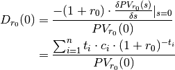
Definition, Macauley Duration:

The Macauley duration or rather the bond duration as defined below is a weighted average of the payment times using the present values of cashflows as weights (this assumes that the cashflows are of same sign)

$D_{r_0}(0) &= \frac{-(1 + r_0) \cdot \frac{\delta PV_{r_0}(s)}{\delta s}|_{s=0}}{PV_{r_0}(0)} \\ &= \frac{\sum^{n}_{i=1}{t_i \cdot c_i \cdot (1 + r_0)^{-t_i}}}{PV_{r_0}(0)}$

Theorem, Reddingtons immunity

When a rate shock (a parallel shift) is added to the calculation rate then the Macauley Duration is the time before the PV for a cashflow $(c_{t_i})$ is risk free, ie the rate shock is absorbed.

Proof:

We look at the future value at time $t_*$ of the present value $PV_{r_0}(0)$ and examine when the future value $(1 + r_0 + s)^{t_*} \cdot PV_{r_0}(s))$ is risk free regarding rate shocks s, ie:

$(\frac{\delta }{\delta s}\left[(1 + r_0 + s)^{t_*} \cdot PV_{r_0}(s)\right])|_{s=0} &= 0 \\ \Updownarrow \\ (\frac{\delta PV_{r_0}(s)}{\delta s} \cdot (1 + r_0 + s)^{t_*} + t_* \cdot (1 + r_0 + s)^{t_* - 1} \cdot PV_{r_0}(s))|_{s=0} &= 0 \\ \Updownarrow \\ (1 + r_0)^{t_* - 1} \cdot (\frac{\delta PV_{r_0}(s)}{\delta s}|_{s=0} \cdot (1 + r_0) + t_* \cdot PV(0)) &= 0 \\ \Downarrow (PV_{r_0}(0) \neq 0)\\ (1 + r_0)^{t_* - 1} \cdot PV_{r_0}(0) \cdot (-D_{r_0}(0) + t_*) &= 0$

So the future value is risk free when $t_* = D_{r_0}(0)$

Q.E.D.

This result is not that important. It shows that the duration is the time before a (parallel) rate shift/shock is absorbed.

It does not show what happens, when PV is 0 which is a problem eg with interest rate swaps.

And it is irrelevant since it would be better to measure eg the time to illiquidity or the value at risk.

The result is only presented for historical reasons.

A bond is itself a portfolio of zero bonds. Since duration and maturity are equal for zero bonds it follows that duration is subadditive, ie the duration of the portfolio is at most the sum of the durations for the parts of the portfolio.

Theorem, Duration for a portfolio

Now the Macauley duration for the sum of two cashflows $(c_{t_i})$ and $(d_{t_i})$ is the present value weighted sum of the durations for each cashflow, ie:

$D_{r_0, c+d}(0) &= \frac{PV_{r_0, c}(0)}{PV_{r_0, c}(0) + PV_{r_0, c}(0)} \cdot D_{r_0, c}(0) + \frac{PV_{r_0, d}(0)}{PV_{r_0, c}(0) + PV_{r_0, d}(0)} \cdot D_{r_0, d}(0)$

An necessary assumption is that all present values $PV_{r_0, c}(0), PV_{r_0, d}(0), PV_{r_0, c+d}(0)$ are nonzero.

Proof:

Now assume two cashflows $(c_{t_i})$ and $(d_{t_i})$ . The present value of the sum of cashflows is the sum of the present values of each cashflow, ie:

$PV_{r_0, c+d}(0) = PV_{r_0, c}(0) + PV_{r_0, d}(0)$

$D_{r_0, c+d}(0) &= \frac{-(1 + r_0) \cdot \frac{\delta PV_{r_0, c+d}(s)}{\delta s}|_{s=0}}{PV_{r_0, c+d}(0)} \\ &= \frac{-(1 + r_0) \cdot (\frac{\delta PV_{r_0, c}(s)}{\delta s}|_{s=0} + \frac{\delta PV_{r_0, d}(s)}{\delta s}|_{s=0})}{PV_{r_0, c+d}(0)} \\ &= \frac{PV_{r_0, c}(0)}{PV_{r_0, c}(0) + PV_{r_0, d}(0)} \cdot D_{r_0, c}(0) + \frac{PV_{r_0, d}(0)}{PV_{r_0, c}(0) + PV_{r_0, d}(0)} \cdot D_{r_0, d}(0)$

Q.E.D.

An similar argument can be made for the modified duration.

This only valid when the PVs $PV_{r_0, c}(0), PV_{r_0, d}(0)$ and their sum $PV_{r_0, c+d}(0)$ are nonzero.

Since there the only elements in the portfolio formula are PVs and durations of each cashflows, the formula can be generalized to when PVs and durations comes from different yieldcurves.

To improve the use of Durations the concept of convexity is introduced.

Definition, Macauley Convexity:

$C_{r_0}(0) &= \frac{(1 + r_0)^2 \cdot \frac{\delta^2 PV_{r_0}(s)}{\delta s^2}|_{s=0}}{PV(0)} \\ &= \frac{\sum^{n}_{i=1}{(t_i+1) \cdot t_i \cdot c_i \cdot (1 + r_0)^{-t_i}}}{PV_{r_0}(0)}$

The rationale for the convexity is following Taylor approximation around s = 0:

$PV_{r_0}(s) &\approx PV_{r_0}(0)\left[1 - \frac{D_{r_0}(0)}{1+r_0} \cdot s + \frac{1}{2} \cdot \frac{C_{r_0}(0)}{(1+r_0)^2} \cdot s^2 \right] \\ & \Downarrow PV_{r_0}(0) \neq 0 \\ \frac{PV_{r_0}(s)}{PV_{r_0}(0)} - 1 &\approx \frac{-D_{r_0}(0)}{1+r_0} \cdot s + \frac{1}{2} \cdot \frac{C_{r_0}(0)}{(1+r_0)^2} \cdot s^2$

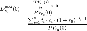
Modified Duration is the elasticy for the present value with regards to to the rate. As can be seen the modified duration is almost the same as the Macauley duration.

Definition, Modified Duration:

$D_{r_0}^{mod}(0) &= \frac{-\frac{\delta PV_{r_0}(s)}{\delta s}|_{s=0}}{PV_{r_0}(0)} \\ &= \frac{\sum^{n}_{i=1}{t_i \cdot c_i \cdot (1 + r_0)^{-t_i - 1}}}{PV_{r_0}(0)}$

And in the modified case it is also possible to define a second order effect, ie a modified convexity.

Definition, Modified Convexity:

$C_{r_0}^{mod}(0) &= \frac{\frac{\delta^2 PV_{r_0}(s)}{\delta s^2}|_{s=0}}{PV_{r_0}(0)} \\ &= \frac{\sum^{n}_{i=1}{(t_i+1) \cdot t_i \cdot c_i \cdot (1 + r_0)^{-t_i - 2}}}{PV_{r_0}(0)}$

To see how modified duration and modified convexity can used to approximate the changes in present value due to rate changes s one has to look at the Taylor approximation of ln(PV):

$\ln(PV_{r_0}(s)) &\approx \ln(PV_{r_0}(0)) - D_{r_0}^{mod}(0) \cdot s + \frac{C_{r_0}^{mod}(0) - D_{r_0}^{mod}(0)^2}{2} \cdot s^2 \\ & \Downarrow PV_{r_0}(0) \neq 0 \\ PV_{r_0}(s) &\approx PV_{r_0}(0) \cdot \exp \left[ - D_{r_0}^{mod}(0) \cdot s + \frac{C_{r_0}^{mod}(0) - D_{r_0}^{mod}(0)^2}{2} \cdot s^2 \right]$

When there is significant curvature/convexity the last approxomation is better. The last approximation does also have a Macauley version:

$PV_{r_0}(s) &\approx PV_{r_0}(0) \cdot \exp \left[ - \frac{D_{r_0}(0)}{1+r_0} \cdot s + \frac{C_{r_0}(0) - D_{r_0}(0)^2}{2 \cdot (1+r_0)^2} \cdot s^2 \right]$

When the present value is zero as might be the case with eg. interest rate swaps other measure are needed.

Below are 2 such measures that tries to handle the problem with zero present values:

Definition, PV01:

Price Value of a 01 (a basis point = 0.0001) is defined as:

$PV01 = (\frac {\partial PV_{r_0}(s)}{\partial s})|_{s=0} \cdot 0.0001$

Definition, PVBP:

Price Value of a Basis Point (= 0.0001) is defined as:

$PVBP = PV_{r_0}(0) - PV_{r_0}(0.0001)$

Using the tangent formula $PV_{r_0}(0.0001) = PV01 + PV_{r_0}(0)$ it is easy to see that the 2 are almost identical (except for the sign).

But here there are no literature suggesting how to handle portfolios. And here is a problem since a basis point might have different probability for different cashflows.

Note

In the Macauley setup presented in most textbooks there is one parameter, the rate, to get a Mark to Market value. This way different cashflows aren’t comparable since they have different rate.

In this presentation the individual rate is split into a common calculation rate $r_0$ and a individual spread s.

This way the Mark to market can be accessed by the spread and portfolio risk can accessed by using risk calculations based on the common rate $r_0$ .

This is a forerunner for the use of yield curves in the risk calculations. One way of seeing the common calculation rate $r_0$ in the next setup is as the constant yield curve.

On the other hand it is obvious that the setup used here contains the classical macauley setup when the common calculation rate is zero, ie $r_0 = 0$

Also it is obvious that the greater spread the less of the market value is explained by the the common calculation rate $r_0$ and hence the greater risk must be associated to such a cashflow.

5.4.2. Fisher-Weil’s Duration and Convexity ¶

Fisher-Weil duration is a refinement of Macauley’s duration which takes into account the yield curve, ie the different prices for different future payments.

Fisher-Weil duration is based on the present values of the cashflows instead of just the payments.

The idea is that in a perfect world a yield curve can return the exact value of a future payment and hence a set of future payments, ie a cashflow.

Using a yieldcurve to get the prices means that if there still is a spread different from zero then it must explain something else, eg the incorporated optionality or the credit risk.

In Addding a Parallel Shift or a spread it is argued that from a mathematical point of view it is better to use a multiplicative spread.

Since the multiplicative spread is more natural using continous forward rates and continous discounting we follow the classical setup we use a yield curve returning the continous forward rate at time t and use continous discounting to get the price.

Definition, Present value, exponential notation:

The Present Value (PV) of a dateflow/cashflow as future payments $(c_{t_i})$ is:

$PV = \sum^{n}_{i=1} c_i \cdot e^{-r_{t_i} \cdot t_i}$

Here the $(r_{t_i})_i$ are the continous forward rates at times $(t_i)_i$

Definition, Multiplicative spread, exponential notation:

The multiplicative spread, s, is a constant added to the continous forward rates. It is an avarage shift that can be used eg for making Mark to market perfect.

Combining the last 2 definitions one gets a formula for the present value of a cashflow, $(c_{t_i})$ , as a function of the multiplicative spread, s:

$PV(s) &= \sum^{n}_{i=1} c_i \cdot e^{-(r_{t_i} + s) \cdot t_i} \\ &= \sum^{n}_{i=1} [c_i \cdot e^{-r_{t_i} \cdot t_i}] \cdot e^{-s \cdot t_i}$

The last derivations shows why the spread is called multiplicative. It is contained in a simple discount factor multiplied to the discounted cashflows.

Note that the spread is similar to the rate in the Uniqueness of the internal rate theorem. So everything said there for the rate goes for the spread as well.

Risk measures from above are defined almost similar as above. Eg we have

Definition, Modified Duration, continous discounting:

$D^{mod}(0) &= \frac{-\frac{\delta PV(s)}{\delta s}|_{s=0}}{PV(0)} \\ &= \frac{\sum^{n}_{i=1}{t_i \cdot [c_i \cdot e^{-r_{t_i} \cdot t_i}]}}{PV(0)}$

The only real problem is how to define Macauley duration and convexity. But here we apply the fact that the multiplicative spread appears as a separate discount factor, so we consider the discounted cashflows by the yieldcurve as the real cashflow. Hence:

Definition, Duration function, continous discounting:

First we define the Duration function:

$D(s) = \frac{-(1 + s) \cdot \frac{\delta PV(s)}{\delta s}}{PV(s)}, PV(s) \neq 0$

And noting that $D(0)$ is both the Macauley and the modified durations (see above). If no yieldcurve is used to discount then $D(r_0)$ is the Macauley duration where $r_0$ is the calculation rate.

And similar:

Definition, Convexity function:

$C(s) = \frac{(1 + s)^2 \cdot \frac{\delta^2 PV(s)}{\delta s^2}}{PV(s)}, PV(s) \neq 0$

Again $C(0)$ is both the Macauley and the modified convexities. And if no yieldcurve is used to discount then $C(r_0)$ is the Macauley convexity where $r_0$ is the calculation rate.

Table Of Contents

Previous topic

Next topic

This Page

5. Thoughts on finance ¶

5.1. On Time, Value and dateflows ¶

5.1.1. Observations and Basic Concepts ¶

5.1.1.1. Observations ¶

5.1.1.2. Time ¶

5.1.1.3. Value ¶

5.1.1.4. The drivers for setting the value of money ¶

5.1.2. The law of one price and dateflows ¶

5.1.3. Discount factor functions ¶

5.1.3.1. On discount factors and rates on a minimum period ¶

5.2. Day count conventions ¶

5.3. On Yieldcurves ¶

5.3.1. Basic concepts ¶

5.3.2. The basic design for yieldcurves ¶

5.3.2.1. continous_forward_rate ¶

5.3.2.2. continous_rate_timeslope ¶

5.3.2.3. instantanious_forward_rate ¶

5.3.2.4. discount_factor ¶

5.3.2.5. zero_coupon_rate ¶

5.3.2.6. discrete_forward_rate ¶

5.3.3. Addding a Parallel Shift or a spread ¶

5.3.4. On the Nelson Siegel yieldcurve ¶

5.3.4.1. Derivation of the Nelson Siegel ¶

5.3.4.2. Calibration ¶

5.3.4.3. Conclusion ¶

5.3.5. On Cubic and Financial Splines ¶

5.3.6. Where to get Yield Curve Data ¶

5.3.7. Yield Curve Derivatives ¶

5.4. A Note on Classical Interest Rate Risk and Risk Management ¶

5.4.1. Present Value, Spread and Risk ¶

5.4.1.1. Evaluation of present value ¶

5.4.1.2. Duration and Convexity ¶

5.4.2. Fisher-Weil’s Duration and Convexity ¶

Navigation

Previous topic

Next topic

This Page

Quick search

Navigation